The Node data table has a number of predefined fields which assist you in quickly analysing various demand (output) scenarios, which might occur in the system. Typically, one such scenario might be the average demand during an average day (ADD). Others might include the average demand over the peak day (PDD), and the demand during the peak hour (PHD). Sometimes, you might also be interested in a fire demand superimposed on the PHD.
Open the Node data table, and navigate to the fields labelled AADD (kL/d) to Th AADD Zone (kL/d). When hovering over these fields, their internal field names will appear, viz. Demand_Scenario1 to Demand_Scenario5. Right-click on the column header for Demand_Scenario1 (alias AADD (kL/d)), and select Configure Columns from the drop-down context menu. This opens the form in which the entire table ‘layout’ can be customised, by defining groups, ordering the columns, setting background colours, numeric formats, alignments, etc.
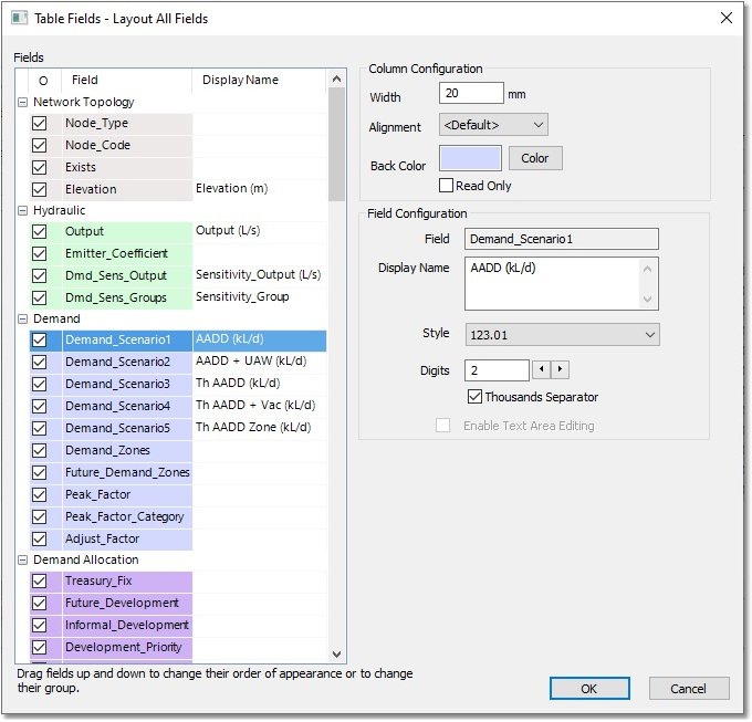
For now, we will only use this form to define new ‘friendly’ display names for the five scenario fields. Change the current Display Name cell of Demand_Scenario1 to ADD_(L/s). Similarly, for Demand_Scenario2, change the Display Name to PDD_(L/s). Do likewise for Demand_Scenario3 (i.e. change the Display Name to PHD_(L/s)), and Demand_Scenario4 (to FIRE_(L/s)). The Display Name cell contents of Demand_Scenario5 can be erased, since it is not applicable to this example. Exit the form by selecting OK, and check in the table that the headers for the Scenario fields have changed.
For this example, let’s assume that the 10 L/s values entered previously for the nodes represent the ADD scenario. Left-click on the column header for the Output (L/s) field to select all the field values in this column, and then use Edit > Copy. Left-click on the column header for Demand_Scenario1, namely the ADD (L/s) column, and use Edit > Paste to copy all the output values into the ADD scenario.
The other scenarios are all related to the ADD scenario by means of ratios. For this example, we will assume that the PDD = 2.0 x ADD. Left-click on the column header for the PDD scenario, and type “=”. Similar to a normal spreadsheet, this opens up the means to type an expression for the values in the cells. You will see the following form, which allows compiling a script to define the values in the cells:
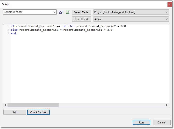
Type in the above query. You can select the fields from the drop-down list, and use the Insert Field button to facilitate the inputting process. Click on the Check Syntax button to check for possible typing/syntax errors. Click on the Run button, and a value of 20 (L/s) = 2.0 x 10 will appear in most cells, except for the top two (which will be zero), where the Demand_Scenario1 values are blank (nil).
For the PHD and FIRE scenarios, perform a similar procedure, but multiply with 4.0, so that their demands are 40 L/s, i.e. 4.0 x ADD.
Note that these formulas are not stored when the script is run; only the calculated values.
Finally, for the FIRE scenario, add 20 L/s fire flow to the 40 L/s PHD value at Node 14, so that the total value is 60 L/s at that node.
It is now very easy to copy and paste the relevant scenario from the scenario fields into the Output (L/s) field, for analysis of the system. For this example, we will be analysing the PHD scenario. Therefore, select this column, and use Edit > Copy. Then, use Edit > Paste to paste the 40 L/s values into the Output (L/s) column.
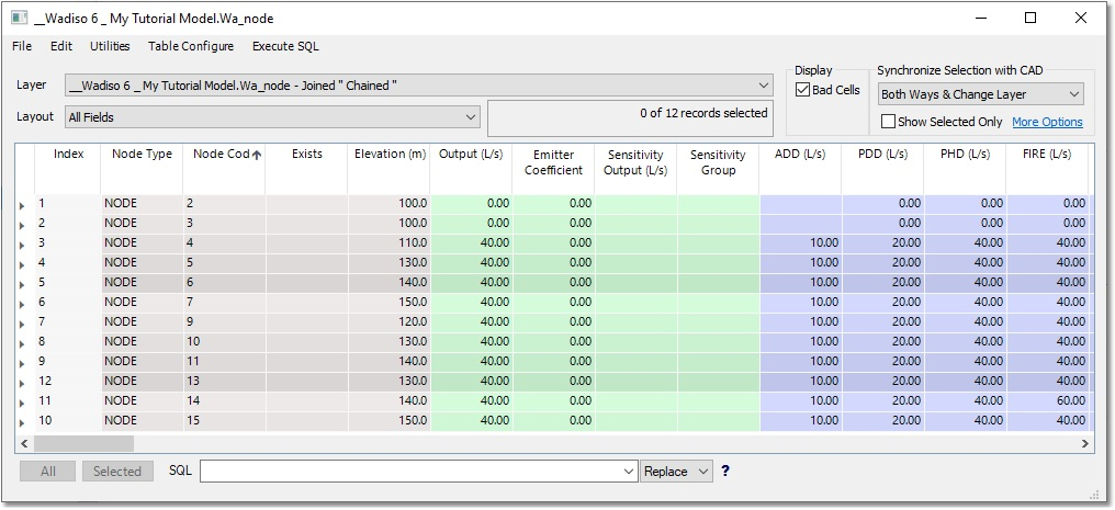
Your final Node table should look like the following:
Whether all of these edits/changes have, in fact, been updated, can also be verified by accessing the Database boxes of some of the nodes in the network.