Database processing forms an integral part of GIS work. It can vary from basic database table field management to complex design of interrelated tables. The spatial data in a GIS must also regularly be updated and managed, e.g. new spatial entities often have to be added/deleted or edited. We will now cover most of these frequently performed data processing tasks.
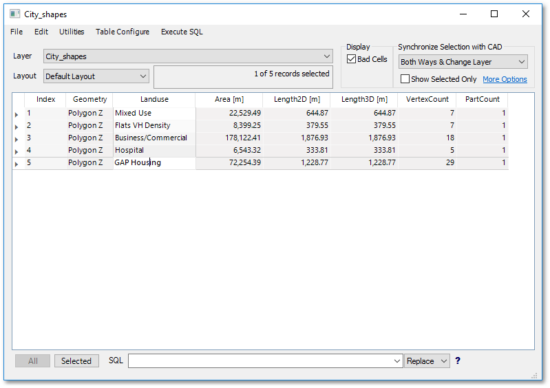
•View the information of the GIS entities by clicking the ![]() Edit Database icon to open the database of the City_shapes GIS layer.
Edit Database icon to open the database of the City_shapes GIS layer.
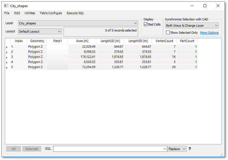
As can be seen from above table, there were five polygon entities created. The fields Area, Length2d, Length3D, VertexCount and PartCount are automatically created system fields that cannot be edited. Field1 is a special user field where you can enter information, which we will discuss hereunder in more detail.
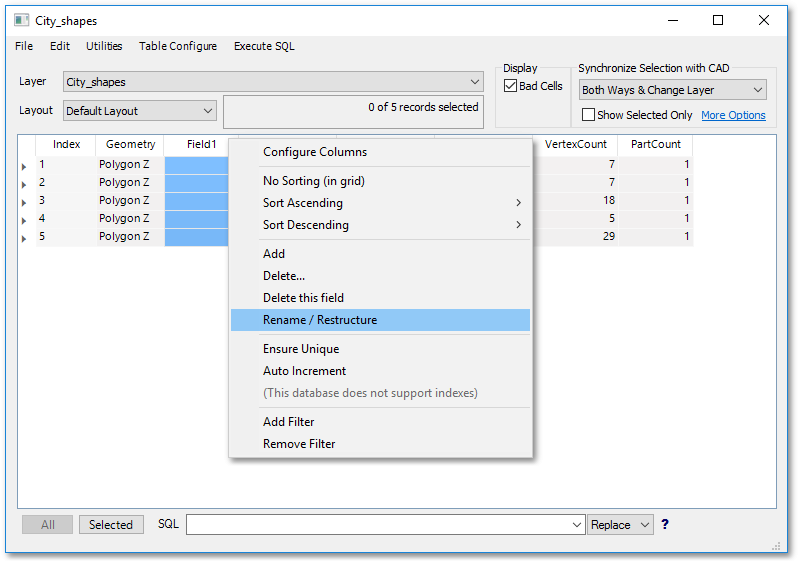
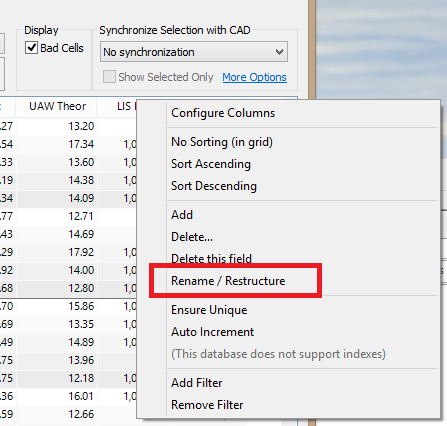
•Change the field (column) name from “Field1” to “Landuse” (Note: the maximum length allowed for a field name is normally 10 characters, with no spaces and special characters are allowed???) and change the field width (max. allowed characters for contents of the field) to 30, by right-clicking on the Field1 field name and select Rename / Restructure from the pop-up menu:
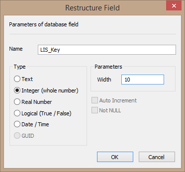
oA window to edit the name and type of information contained in the field (column) pops up:
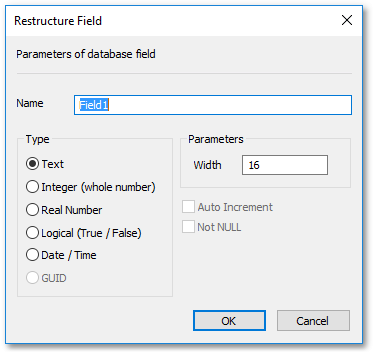
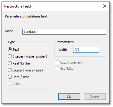
oChange the name to “Landuse” and change the width (allowed characters) to 30:
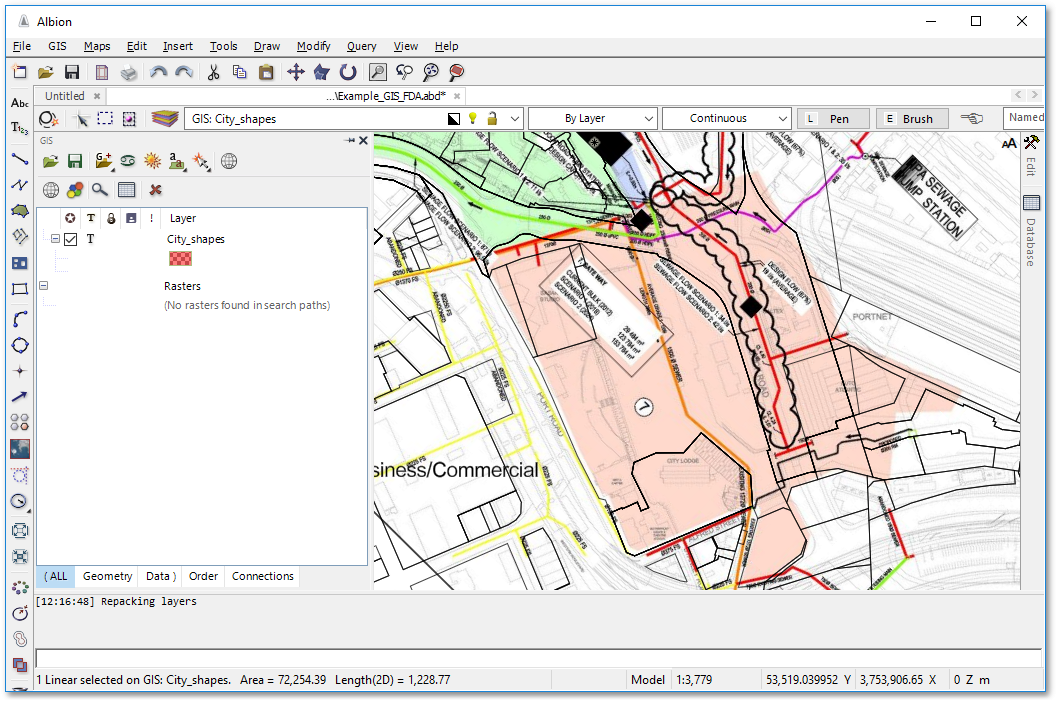
•Enter the landuse of the entities (located on the CAD- City Bowl FDA layer as text labels). Note, switch on the visibility of this layer if it is currently invisible.
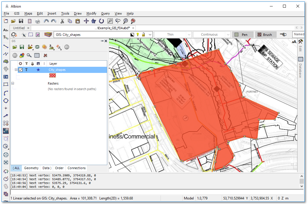
•To create additional entities on the newly created City_shapes GIS layer, make this layer current and click the ![]() Create a polygon tool from the left vertical toolbar. You can now start capturing e.g. the waterfront future areas by tracing over the waterfront FDA background image layer (you may have to switch on the visibility of the waterfront FDA background image layer if it is currently off).
Create a polygon tool from the left vertical toolbar. You can now start capturing e.g. the waterfront future areas by tracing over the waterfront FDA background image layer (you may have to switch on the visibility of the waterfront FDA background image layer if it is currently off).
A new polygon entity on the City_shapes GIS layer is created:
•Open the edit data table by clicking the ![]() Edit Database icon. A new record (row) has been created, with landuse field at this stage blank.
Edit Database icon. A new record (row) has been created, with landuse field at this stage blank.
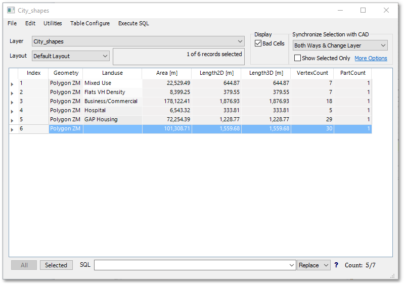
You can enter for the above record the following landuse type: "Business/Commercial". On a later stage, you can continue with capturing all the other future development areas from the image and fill in their land use as “Business/Commercial”, as described above.
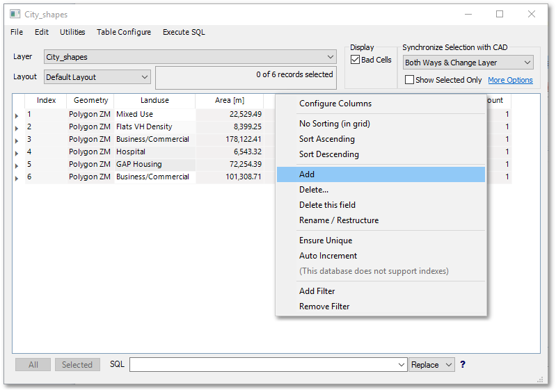
oCreate new fields called “Units” and “AADD”. This can be accomplished by right-clicking at the top (the field name bar) and select Add.
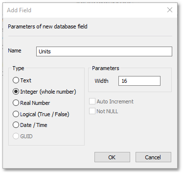
oCreate a field called “Units”, with Type: Integer (whole number)
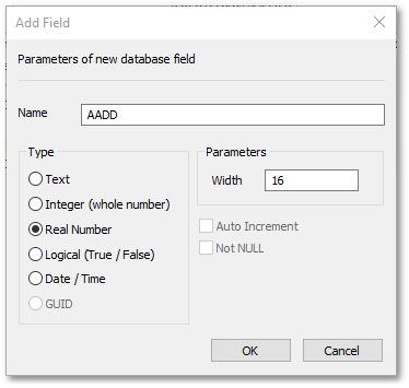
oCreate a field called “AADD”, with Type: Real Number
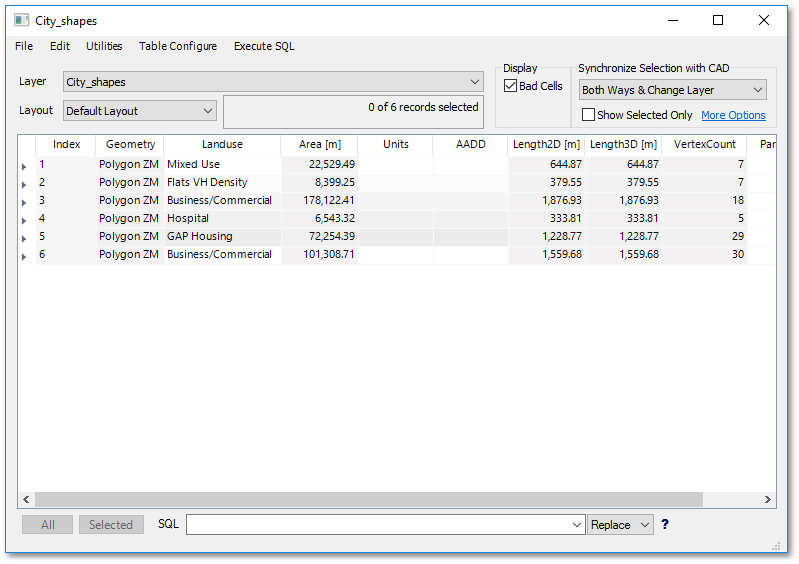
Two new field have been created that can be filled.
You can now save the changes made to the City_shapes file by clicking on the blue star (i.e. modified icon) in the GIS Layer Manager box and then click on the Save Changes button of the ensuing Save/Discard Tables dialog box. This part of the tutorial is finished for now - we will continue with data processing, but with new example data.
oRemove all GIS files from the project: highlight the City_shapes file in the GIS Layer Manager box (which should be the only shapefile in the list), by right-clicking on it, and selecting Remove from the pop-up menu.
oRemove the drawing file Example_GIS_FDA.abd from the project: File > Close Drawing
oWe can now continue to load in treasury data containing water demand readings (that are often managed in Excel spreadsheets).
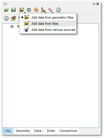
oThe treasury data can be exported from Excel to a .csv (Comma Separated Values) file. This file can then be loaded into Albion by clicking the ![]() Add Data icon in the GIS Layer Manager box, and then selecting the Add data from files pop-up menu item:
Add Data icon in the GIS Layer Manager box, and then selecting the Add data from files pop-up menu item:
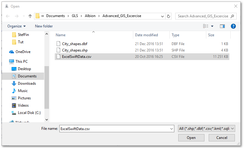
oFrom the Open dialog box, select the file ExcelSwiftData.csv:
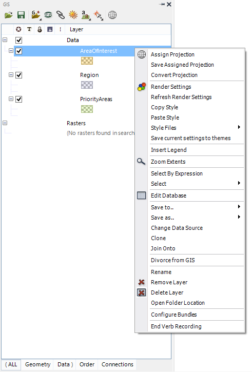
oRight-click on imported *.csv layer (viz. ExcelSwiftData) and select Save As>Save Layer As..., browse, select your user folder and save database as Xbase type “SWIFT TABLE BAY.dbf” (note, the newly created file will automatically be loaded into Albion and appear in the GIS Layer Manager):
o The database format (.dbf) is the recommended format to use for managing data tables in Albion - the .csv is too slow and is only a temporary measure during the importing process. Remove ExcelSwiftData.csv by right-clicking on it, and selecting Remove from the pop-up menu.
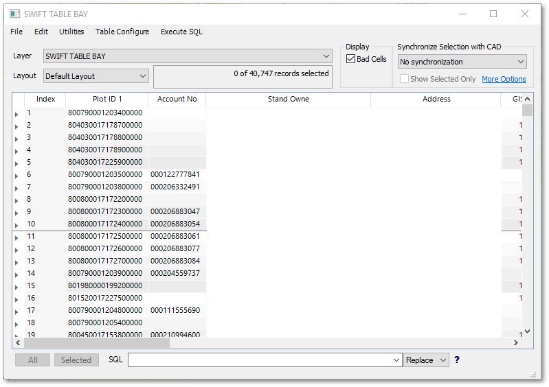
oThe “SWIFT TABLE BAY.dbf” table can now be opened for viewing by clicking the ![]() Edit Database icon in the GIS Layer Manager box.
Edit Database icon in the GIS Layer Manager box.
oWe not want to change the data type of the LIS_Key field to integer. This will ensure we can perform a proper join with another shape file later
oRight-click on the LIS_Key heading near the far right, then select Rename / Restructure from the pop-up menu:
oThen select Integer and a Width of 10, followed by OK:
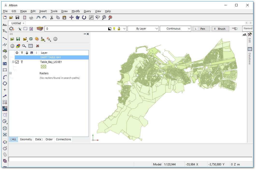
oWe can now open the shapefile "Table_Bay_LIS_KEY.shp" which contain parcel polygons for the table bay study area.
oNow open the table behind the shapefile for viewing and Rename/Restructure the LIS_Key for this table to Integer and a Width of 10, in the same way as previously done for “SWIFT TABLE BAY.dbf”
oThe next step is to create a joined table containing information from both the database table of the shapefile "Table_Bay_LIS_KEY.shp" (left table, see screen-shot below) and the SWIFT TABLE BAY.dbf (right) table. The two tables will be linked via the common field LIS_Key, which contains unique identification codes. Hereby a one-to-one relationship can be built between the records of the two tables based on the matching identification codes.
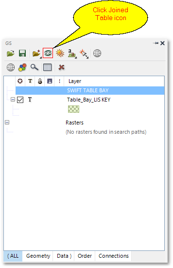
oClick in the GIS Layer Manager box on the ![]() Create Joined Table icon to open the Create Joined Table box:
Create Joined Table icon to open the Create Joined Table box:
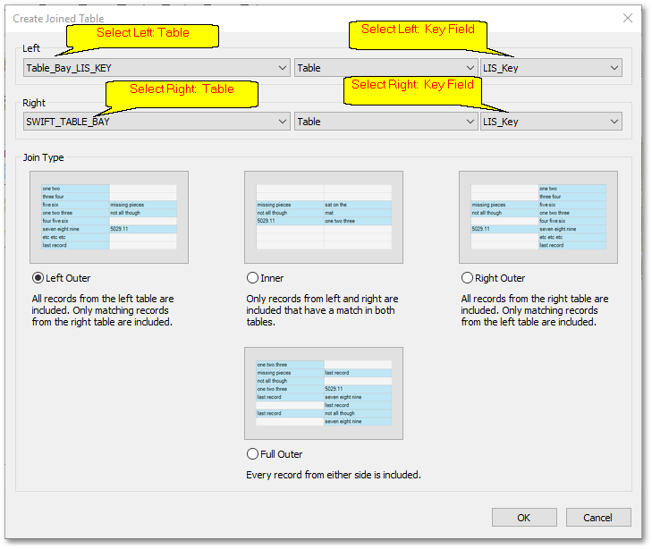
oSelect Left table: Table_Bay_LIS_KEY, Right Table: SWIFT TABLE BAY, Fields to join on (LIS_Key), Join Type: Left Outer and finally, Click OK. Note, a virtual layer viz. Table_Bay_LIS_KEY => SWIFT TABLE BAY (i.e. memory only) will automatically be created containing the output of the join operation and will be listed in the GIS Layer Manager.
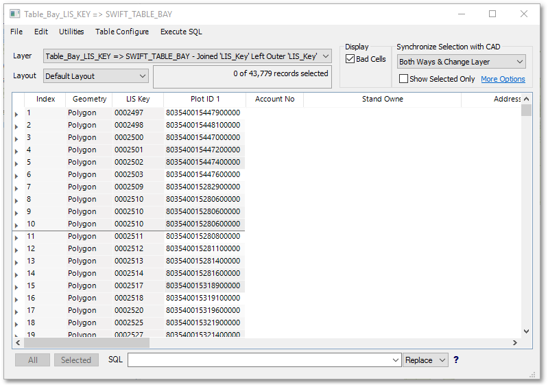
oCheck joined database table of the Table_Bay_LIS_KEY => SWIFT TABLE BAY by clicking on the ![]() Edit Database icon in the GIS Layer Manager.
Edit Database icon in the GIS Layer Manager.
oSave the joined data of the Table_Bay_LIS_KEY => SWIFT TABLE BAY layer as a new shapefile by right-clicking on it in the GIS Layer Manager and select Save As>Save Layer As... from the pop-up menu. Specify a new file name: “Table_Bay_Swift.shp”.
This concludes the database processing and spatial data editing part of the tutorial. The next part will focus on exploring spatial data results by applying special querying and rendering functionality.