All the data required for the hydraulic analysis of the existing system has now been captured. The data is resident in a SQLite geodatabase (resident only in program memory, because not saved yet), for which the location was previously specified.
The data is kept in six different ‘categories’, namely Pipe data, Pump data, Valve data, Tank data, Node data, and Appurtenance data. A grid table for each of these categories can be opened for viewing the data (and results), and for further editing, if required. This is done by selecting Model Data > Model Tables, and then from the sub-menu, selecting one of the following items: Pipe/CV, Pump, Valve, Node or Tank. (There is also an option to load a Curve grid table, which is for advanced use of the program, where special pump curves and tank volume versus water level curves apply. This is not addressed in this tutorial).
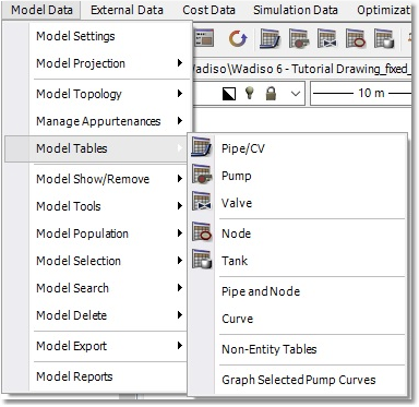
Open the Pipe/CV table under Model Data > Model Tables > Pipe/CV. This table provides a list of all the pipes in the system, i.e. a sub-set of all the links in the model. (The ‘CV’ stands for ‘Check Valve’, which is a special type of pipe that allows flow in only one direction). In this table, all the data (and results if available) associated with the pipes are shown, e.g. their diameters, lengths and Hazen-Williams roughness coefficients (or Darcy-Weisbach absolute roughness).
Browsing through the table will reveal that the various columns/fields are grouped together in categories (displayed in distinctive colours), corresponding exactly to the various groups and fields found in the Database box of an individual pipe. The grouping of fields and the formatting of the display (numeric format, background colour) can be set as a table ‘Layout’, that can be saved and later retrieved. A variety of such layouts are predefined and loaded at program installation, e.g. a “Data” layout focusing on the input data, a “Results” layout focusing on the flows and pressures, etc. Regular Wadiso users can pick an appropriate layout, and do not have to bother with creating and specifying their own customised layout.
In the “All Fields” layout, the first five columns display the Network Topology info, i.e. Link Type, Link Code, From Code, To Code and Exists. The next six Hydraulic columns are the system data fields, required for hydraulic calculations. Then, there are Physical, Descriptive, Location, Results, Planning and Assets groups. These are followed by Time Simulation and Optimization groups, related to the respective specialised modules of the program. The final four groups are: Integrity, GUID and Geometry, Model Functions, and lastly Demand Allocation. The latter, viz. Demand Allocation columns, relate to the integration with the Swift™ water demand modelling program.
As shown before, this Pipe/CV table can be used to change/edit any of the data fields associated with the pipes in the system. This is another method, in addition to the individual editing of specific pipes in the CAD/GIS environment. The table is very similar to any commercial spreadsheet, in that columns can be formatted and hidden, and that values can be copied and pasted, or temporary scripts can be entered and executed to update values. For instance, what we will do here is to change the Hazen-Williams coefficient of the PVC pipes in the network (i.e. Pipes 5 to 18), from the current (default) values of 100, to 115. In the table, navigate to the cell representing the HW Coeff of Pipe 5 (i.e. the Friction Coefficient field value), and change it to 115. Then, select Edit > Copy (or Ctrl + C). Now, mark (with click-hold-drag) the Friction Coefficient cells of Pipes 6 to 18, and select Edit > Paste (or Ctrl + V). Pipes 5 to 18 now have a HW Coeff value of 115.
This change (and any other changes made in the table) will only be updated permanently to the geodatabase when the table is closed, and the model is saved. The table can be closed by clicking on the ![]() Close icon in the top right-hand corner of the table window, or by selecting File > Close. From the main menu, select Manage Models > Save Model, followed by selecting Yes, to confirm saving the HW Coeff change to the geodatabase.
Close icon in the top right-hand corner of the table window, or by selecting File > Close. From the main menu, select Manage Models > Save Model, followed by selecting Yes, to confirm saving the HW Coeff change to the geodatabase.
Open the Node table under Model Data > Model Tables > Node. This table provides a list of all the ordinary nodes (junctions) in the system, i.e. a sub-set of all the nodes in the model. In this table, the data associated with the ordinary nodes are shown, e.g. their outputs. Browsing through the table will reveal that the various columns/fields are grouped together in categories (displayed in distinctive colours), similar to the various groups and fields found in the Database box of an individual node. As for the pipe table (and, in fact, any table in the model or in the GIS environment), the grouping of fields and the formatting of the display (numeric format, background colour) can be set as a table ‘Layout’, that can be saved and later retrieved. A variety of such layouts are predefined and loaded at program installation.
In the “All Fields” layout, the first four columns display the Network Topology info, i.e. Node Type, Node Code, Exists and Elevation (m). The next four Hydraulic columns are the system data, required for hydraulic calculations, such as the Output (L/s) field. The Demand columns contain demand (output) scenarios, which can be copied to the aforementioned Output (L/s) column, in order to analyse the various scenarios (more about this later). Then, there are Demand Allocation, Physical, Descriptive, Location, Results and Assets groups. These are followed by Time Simulation and Optimization groups, related to the respective specialised modules of the program. The final three groups are: Integrity, GUID and Geometry, and lastly Model Functions.
All six of the data tables can be used to edit system info, and can be customised to the user's preferences with regard to which columns should be visible, number formats, font sizes, colours, etc. Any edits/changes made in the tables, when updated to program memory, will also be reflected in the Albion environment, and in the individual node and link Database boxes.