The Wadiso program can produce X-Y type graphs of the following data and results:
•Model Data & Results
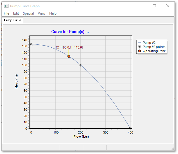
- Pump characteristic curves, can be viewed for a selected the pump link via Model Data > Model Table > Graph Selected Pump Curves or by right-clicking on the pump link and use Selected Pumps (1) > Graph pump curves. Note if the system is balanced, then the balanced operating point for the pump is also shown, see below.
- Curves, i.e. Multipoint pump curves (Flow vs. Head), Pump efficiency curves (Flow vs. %), Tank Volume curves (Tank height vs. volume) and GPV head loss curves (Flow vs. head loss). Graphs of these curves are accessible from the Curve Data table.
•Time /WQ Simulation Data
-Time pattern, accessible from the Water Time Simulation Data table. Two types can be plotted, viz. a plot of the pattern as specified, and a plot of the pattern extended over the total duration of the time simulation, after application of multipliers. Time patterns are used to model fluctuating demands, pump scheduling, varying energy price over time, reservoir head variations over time and water quality source variations over time.
•Time/WQ Simulation results
- For Nodes, the time series of water demand, energy grade line, pressure head and water quality are plotted. Time series graphs for nodes are accessible after time/WQ simulation from the the right-click menu of the node, or via Analysis > Time Simulation > Result Tables > Result Nodes.
- For Tanks/Reservoirs, the time series of inflow(+)/outflow(-), energy grade line, water level and water quality are plotted. Time series graphs for tanks are accessible after time/WQ simulation from the right-click menu of the tank/reservoir, or via Analysis > Time Simulation > Result Tables > Result Nodes.
- For Pipes/CV, the time series of flow, velocity, head loss energy gradient and water quality are plotted. Time series graphs for pipes/CV are accessible after time/WQ simulation from the right-click menu of the pipe/CV, or via Analysis > Time Simulation > Result Tables > Result Graphs.
- For Pumps, the time series of flow, head loss, power and water quality are plotted. Time series graphs for pumps are accessible after time/WQ simulation from the right-click menu of the pump, or via Analysis > Time Simulation > Result Tables > Result Graphs.
- For Valves, the time series of flow, velocity, head loss and water quality are plotted. Time series graphs for valves are accessible after time/WQ simulation from the right-click menu of the valve, or via Analysis > Time Simulation > Result Tables > Result Graphs.
•Cost and Optimization Data
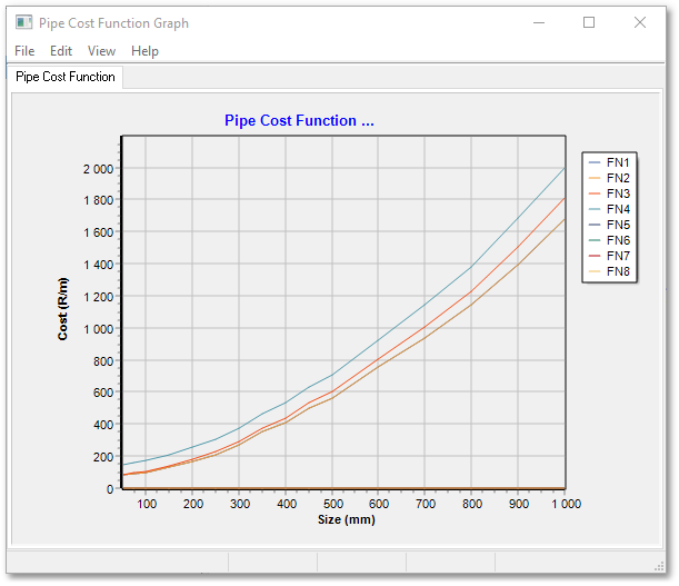
- For Pipe Cost Functions, a graph of diameter vs. unit cost (Monetary Unit per length, e.g. R/m). Graphs of the pipe cost functions can be viewed by using the Cost Data > Cost Data Graphs > Pipe.
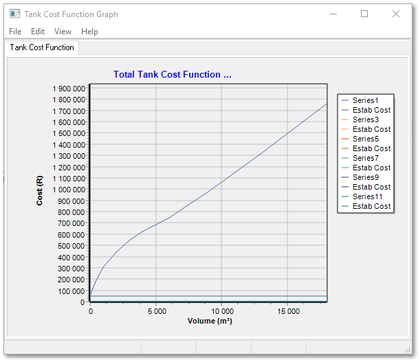
- For Tank Cost Functions, a tank volume vs. total cost (Monetary, e.g. R). Graphs of the tank cost functions for the various tank types can be viewed via Cost Data > Cost Data Graphs and then select from the sub-menu one of the following: Ground Level Tank (Tank), Elevated Tank (Tower), or Beak Pressure Tank (BPT).
- For Consumption characteristics used for tank sizing, three graphs are accessible from the Tank Sizing Parameters Editor. These are:
i) The 24 hour demand pattern;
ii) The 168 hour peak week demand pattern;
iii) The Peak Factor curve, i.e. Peak demand factors vs. Peak period.
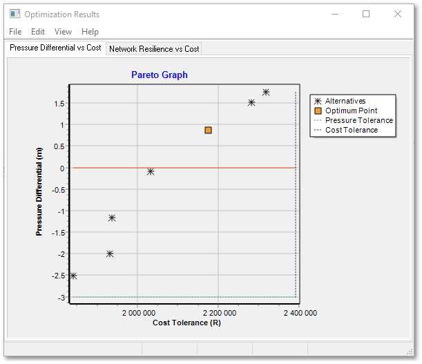
•Optimization results
- A graph plotting cost vs. pressure for the optimum solution and the list of Pareto Optimal solutions is available via the Analysis > Optimization > Optimization Graph menu option.